Static malware analysis using machine learning techniques
Machine learning–driven static malware analysis of Windows PE files, applying XGBoost and DNN models on extracted headers, sections, import tables, strings, byte patterns to detect malicious binaries.
The digital threat landscape is continuously expanding, with new and sophisticated malware variants appearing daily. Traditional malware detection methods, primarily relying on static signatures, struggle to identify these rapidly evolving threats and zero-day exploits. Static analysis, which examines suspicious files without execution, offers a safe and efficient alternative to dynamic analysis. However, the sheer volume and complexity of modern malicious code necessitate automated approaches. Machine learning provides powerful tools to analyze static file characteristics and identify potential malware. This article explores the application of machine learning techniques to static malware analysis of Windows Portable Executable (PE) files, focusing on the capabilities of XGBoost and Deep Neural Networks (DNNs) in this critical security domain. The dataset used for this analysis, along with the scripts for feature extraction, are publicly available at https://github.com/arxlan786/Malware-Analysis/tree/master. Furthermore, the implementations of the machine learning models discussed can be found in the following Kaggle notebook: https://www.kaggle.com/code/mateistoian/static-mallware-anallisys.
Windows PE Files: The Source of Static Features
Windows Portable Executable (PE) files are the standard format for executables, dynamic-link libraries (DLLs), and other executable code on the Windows platform. Understanding the structure of PE files is fundamental for static malware analysis. By examining the internal organization and metadata of a PE file without executing it, security analysts and automated systems can gather crucial information about its potential functionality and intent.
Static feature extraction from PE files involves programmatically analyzing different parts of the file structure. Key areas of analysis include:
- PE Headers: These contain vital metadata about the file, such as timestamps, entry points, and the sizes and locations of various file sections.
- Section Information: PE files are divided into sections (like
.textfor code,.datafor initialized data, etc.). Analysis includes examining section names, sizes, permissions (indicating if a section is executable or writable), and entropy (high entropy can suggest packed or encrypted malicious content). - Import and Export Directories: These tables list the functions a program imports from external libraries (like Windows APIs) or exports for use by other programs. The specific APIs a program intends to use can be a strong indicator of its behavior, malicious or otherwise.
- Strings: Human-readable strings embedded in the file can reveal command-and-control server URLs, file paths, or other suspicious information.
- Byte Sequences: Analyzing patterns in the raw bytes can sometimes reveal characteristics of malicious code, even if obfuscated.
These extracted features, which represent the static properties of the PE file, serve as the input data for machine learning models. By learning the patterns within these features that differentiate known malware from benign software, ML models can effectively classify new, unseen files.
Machine Learning Approach 1: XGBoost
Our first machine learning approach utilizes Extreme Gradient Boosting, commonly known as XGBoost. XGBoost is a highly efficient and powerful open-source library that implements the gradient boosting framework. It's an ensemble learning method that builds a series of decision trees sequentially. Each new tree in the sequence is trained to correct the errors made by the previous trees, iteratively improving the model's overall performance. This boosting technique, combined with various regularization strategies to prevent overfitting, makes XGBoost a robust choice for classification tasks.
In the context of static malware analysis, XGBoost takes the extracted static features from the PE files (as discussed in Section 2) as input. It learns complex relationships and patterns within these features through its ensemble of decision trees. The model effectively partitions the feature space based on the learned patterns, ultimately making a decision on whether a given PE file is likely malicious or benign.
For our experiments, the XGBoost model was configured with the following key hyperparameters:
-
n_estimators=1000: The number of boosting rounds or trees to build. A higher number can lead to better performance but increases training time and risk of overfitting. -
max_depth=10: The maximum depth of each individual decision tree. This controls the complexity of the trees. -
subsample=0.8: The fraction of samples used to train each tree. This helps prevent overfitting by introducing randomness. -
colsample_bynode=0.9: The fraction of features used when building each tree's nodes. This also helps prevent overfitting. -
random_state=42: A seed for reproducibility. -
n_jobs=-1: Utilizes all available CPU cores for parallel processing, speeding up training.
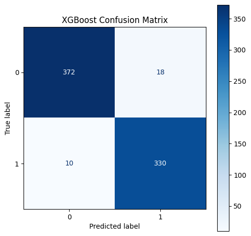
After training the XGBoost model on our dataset, we evaluated its performance on the held-out test set. The results are summarized in the classification report and AUC score below:
| precision | recall | f1-score | support | |
|---|---|---|---|---|
| 0 | 0.97 | 0.95 | 0.96 | 390 |
| 1 | 0.95 | 0.97 | 0.96 | 340 |
| accuracy | 0.96 | 730 | ||
| macro avg | 0.96 | 0.96 | 0.96 | 730 |
| weighted avg | 0.96 | 0.96 | 0.96 | 730 |
XGBoost AUC: 0.991975867269985
The classification report shows strong performance across all metrics. For the malicious class (1), the model achieved a precision of 0.95, meaning 95% of files predicted as malicious were indeed malicious. It also achieved a recall of 0.97, indicating it correctly identified 97% of the actual malicious files in the test set. The overall accuracy was 0.96, and the F1-score for both classes was 0.96, demonstrating a good balance between precision and recall. The high AUC score of 0.992 further confirms the model's excellent ability to discriminate between benign and malicious PE files.
Pros of using XGBoost for this task:
-
High Performance: XGBoost is known for achieving state-of-the-art results on many tabular datasets, including those derived from static analysis features.
-
Handles Various Feature Types: It can effectively work with a mix of numerical and categorical features commonly found in PE file analysis.
-
Built-in Regularization: Its regularization techniques help prevent overfitting, which is crucial given the potentially high-dimensional nature of static features.
-
Feature Importance: XGBoost can provide insights into which features were most important for the classification decision, aiding in understanding the characteristics that indicate malware.
-
Efficiency: It is optimized for speed and performance, making training relatively fast.
Cons of using XGBoost:
-
Hyperparameter Tuning: Optimal performance often requires careful tuning of numerous hyperparameters.
-
May Not Capture Complex Spatial/Sequential Patterns: While powerful, XGBoost primarily works on tabular data and may not inherently capture complex spatial relationships (like in image representations of binaries) or sequential dependencies (like in instruction sequences) as effectively as some deep learning architectures designed for such data.
-
Interpretability (relative to single trees): While it provides feature importance, understanding the decision process of the entire ensemble can be less intuitive than a single decision tree.
Machine Learning Approach 2: Deep Neural Networks (DNN)
Our second approach employs Deep Neural Networks (DNNs). DNNs are a class of artificial neural networks characterized by multiple layers between the input and output layers. These hidden layers allow DNNs to learn complex, hierarchical representations of the input data, automatically discovering intricate patterns that might not be immediately obvious through manual feature engineering or simpler models. This ability to learn abstract features makes DNNs powerful for tasks involving complex data like those derived from binary files.
For this task, we designed a feedforward DNN architecture specifically for processing the tabular static features extracted from the PE files. The architecture consists of several densely connected layers, incorporating techniques to improve training stability and prevent overfitting:
-
Input Layer: Receives the vector of static features extracted from each PE file. The size of this layer is determined by the
input_dim, which corresponds to the number of features. -
Hidden Layers: Three hidden layers are used to process the input features and learn increasingly abstract representations.
-
The first hidden layer has 128 neurons.
-
The second hidden layer has 64 neurons.
-
The third hidden layer has 32 neurons.
-
Each hidden layer is followed by:
-
nn.BatchNorm1d: Batch normalization layers are used to normalize the inputs to the activation functions, which helps stabilize and accelerate the training process. -
F.relu: The Rectified Linear Unit (ReLU) activation function introduces non-linearity, allowing the network to learn complex, non-linear relationships in the data. -
nn.Dropout(0.3): Dropout layers randomly set 30% of the input units to zero during training. This acts as a regularization technique, preventing co-adaptation of neurons and reducing overfitting.
-
-
-
Output Layer: A single neuron with a linear activation function (
nn.Linear(32, 1)) is used to produce a single output value. This output is then typically passed through a sigmoid function (often implicitly handled by the loss function) to produce a probability score between 0 and 1, representing the likelihood of the file being malicious.
The DNN model was trained using the following configuration:
-
Loss Function:
nn.BCEWithLogitsLoss(Binary Cross-Entropy with Logits Loss). This loss function is suitable for binary classification and is numerically more stable than applying a sigmoid followed by standard BCE. Thepos_weightargument was used, likely to address potential class imbalance in the dataset by giving more importance to the minority class (often the malicious samples). -
Optimizer:
optim.Adam. The Adam optimizer is an adaptive learning rate optimization algorithm that is widely used and generally performs well. -
Learning Rate:
lr=0.0001. A small learning rate was chosen to allow the model to converge steadily. -
Number of Epochs:
num_epochs = 1000. The model was set to train for a maximum of 1000 epochs. -
Early Stopping: A
patienceof 10 was implemented. Training would stop if the validation loss did not improve for 10 consecutive epochs, preventing overfitting and saving computational resources.
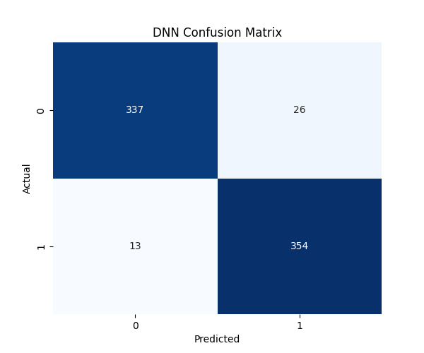
After training, the DNN model's performance was evaluated on the test set, yielding the following results:
| precision | recall | f1-score | support | |
|---|---|---|---|---|
| 0.0 | 0.97 | 0.91 | 0.94 | 363 |
| 1.0 | 0.92 | 0.97 | 0.94 | 367 |
| accuracy | 0.94 | 730 | ||
| macro avg | 0.94 | 0.94 | 0.94 | 730 |
| weighted avg | 0.94 | 0.94 | 0.94 | 730 |
The DNN achieved an overall accuracy of 0.94 and an F1-score of 0.94 for both classes. It demonstrated a high recall of 0.97 for the malicious class (1.0), indicating it was very effective at identifying actual malware, similar to the XGBoost model. The precision for the malicious class was 0.92. The AUC score of 0.988 also indicates strong discriminative power.
Pros of using DNNs for this task:
-
Automatic Feature Learning: DNNs can automatically learn complex, non-linear patterns and interactions within the static features without requiring explicit feature engineering beyond the initial extraction.
-
Potential for Higher Accuracy: With sufficient data and appropriate architecture, DNNs can potentially achieve very high accuracy by capturing intricate relationships.
-
Adaptability: The architecture can be modified to potentially handle different types of static data representations, such as treating byte sequences as time series or binary images.
Cons of using DNNs:
-
Data Requirements: DNNs typically require large amounts of labeled data to train effectively and avoid overfitting.
-
Computational Cost: Training DNNs can be computationally expensive and time-consuming, requiring specialized hardware like GPUs.
-
Black Box Nature: DNNs are often considered "black boxes," making it difficult to interpret why a specific prediction was made, which can be a drawback in security analysis where understanding the indicators of compromise is valuable.
-
Hyperparameter Sensitivity: Performance is highly dependent on the architecture design and hyperparameter tuning.
Comparative Analysis: XGBoost vs. DNN for Static Malware Detection
Having explored the application and performance of both XGBoost and Deep Neural Networks for static malware detection based on PE file features, we can now conduct a comparative analysis of their effectiveness and characteristics.
Looking at the classification reports and AUC scores from our experiments:
| Metric | XGBoost | DNN |
|---|---|---|
| Accuracy | 0.96 | 0.94 |
| Precision (0) | 0.97 | 0.97 |
| Recall (0) | 0.95 | 0.91 |
| F1-score (0) | 0.96 | 0.94 |
| Precision (1) | 0.95 | 0.97 |
| Recall (1) | 0.97 | 0.94 |
| F1-score (1) | 0.96 | 0.94 |
| AUC | 0.992 | 0.988 |
Based on these results, the XGBoost model slightly outperformed the DNN in overall accuracy (0.96 vs 0.94) and achieved a marginally higher AUC score (0.992 vs 0.988). Both models demonstrated very high recall for the malicious class (0.97 for XGBoost, 0.94 for DNN), indicating they were both effective at identifying the vast majority of actual malicious files. XGBoost showed slightly better precision for both classes and higher recall for the benign class (0).
The slightly superior performance of XGBoost in this specific experiment could be attributed to several factors. XGBoost, as a tree-based ensemble method, is often very effective on tabular data with a mix of feature types, which is characteristic of the static features extracted from PE files. Its boosting mechanism and regularization techniques are well-suited to handling potentially complex interactions between these features. While DNNs are powerful at learning hierarchical representations, the specific architecture used here, a relatively simple feedforward network, might not have fully captured all the nuances in the tabular PE features compared to the complex decision boundaries created by the XGBoost ensemble. Additionally, the performance of DNNs can be highly sensitive to architecture and hyperparameters, and further tuning might potentially improve the DNN's results.
Beyond raw performance metrics, there are practical trade-offs to consider:
- Training Time and Resources: DNNs, especially larger or more complex architectures, typically require significantly more computational resources (often GPUs) and longer training times compared to XGBoost, which can be efficiently trained on CPUs and is generally faster for datasets of this size.
- Inference Speed: Once trained, both models can generally provide fast predictions, which is crucial for real-time malware scanning. The speed depends on the model size and the hardware used.
- Interpretability: XGBoost offers insights into feature importance, allowing us to understand which PE file characteristics the model found most predictive of maliciousness. DNNs, on the other hand, are often considered "black boxes," making it difficult to interpret the reasoning behind a specific classification. This lack of interpretability can be a disadvantage in security analysis where understanding why a file is flagged as malicious is important for investigation and threat intelligence.
- Feature Engineering: XGBoost can leverage well-engineered features effectively. While DNNs can learn features automatically, the quality of the initial extracted features still significantly impacts their performance.
In summary, both XGBoost and the implemented DNN demonstrated strong capabilities for static malware detection using PE file features. XGBoost showed slightly better overall performance in this comparison, potentially due to its suitability for the nature of the data. However, the choice between the two (or using both) depends on the specific requirements of the application, including performance needs, available computational resources, and the importance of model interpretability.
Possible Improvements and Future Directions
The application of machine learning to static malware analysis is a continuously evolving field, and there are numerous avenues for improving the models and techniques discussed. Based on our exploration, here are some possible improvements and future directions:
- Advanced Feature Engineering: While the current set of static features from PE files is effective, exploring more sophisticated feature engineering techniques could yield better results. This might include:
- Analyzing the sequence of imported API calls using techniques like n-grams or sequence-based models.
- Extracting and analyzing control flow graphs or function call graphs statically.
- Converting binary files into image representations and using Convolutional Neural Networks (CNNs) to learn spatial patterns.
- Analyzing the opcode sequences within the code sections.
- Exploring Other Machine Learning Models: Investigating other powerful machine learning algorithms could be beneficial. This includes:
- Other ensemble methods like LightGBM or CatBoost.
- Support Vector Machines (SVMs) with different kernels.
- More complex or specialized deep learning architectures, such as Recurrent Neural Networks (RNNs) for sequential data (like API calls or byte sequences) or Graph Neural Networks (GNNs) for analyzing structural relationships in PE files.
- Ensemble Methods: Combining the predictions of multiple models (e.g., an ensemble of XGBoost and DNN, or multiple instances of the same model trained differently) can often lead to more robust and accurate results than using a single model.
- Addressing Data Challenges: Malware datasets often suffer from class imbalance (many more benign samples than malicious ones) and concept drift (malware tactics and techniques change over time). Future work could focus on:
- Implementing advanced data balancing techniques (e.g., SMOTE, undersampling).
- Developing methods for continuous model retraining or adaptive learning to handle concept drift.
- Curating larger and more diverse datasets.
- Explainable AI (XAI): Given the "black box" nature of some models, particularly DNNs, incorporating XAI techniques (like SHAP or LIME) to understand which features contribute most to a prediction can enhance trust and aid security analysts in their investigations.
- Integration with Dynamic Analysis: While this article focuses on static analysis, a hybrid approach combining static and dynamic analysis features can provide a more comprehensive view of a file's potential maliciousness and improve detection rates.
- Efficiency and Scalability: For real-world deployment, optimizing models for faster inference and ensuring the entire pipeline can handle a high volume of files is crucial. This might involve model quantization, pruning, or distributed computing.
By pursuing these avenues, the effectiveness and practicality of machine learning-based static malware analysis can be further enhanced, contributing to stronger defenses against the ever-evolving threat landscape.
Conclusion
In this article, we explored the application of machine learning techniques to the critical task of static malware analysis, focusing on the widely used Windows Portable Executable (PE) file format. We discussed how analyzing the structure and features of PE files without execution provides valuable insights into potential malicious behavior and serves as the foundation for ML-driven detection.
Our comparative analysis of XGBoost and Deep Neural Networks (DNNs) demonstrated that both approaches are highly effective in distinguishing between benign and malicious PE files based on static features. While XGBoost showed slightly superior performance in our specific experimental setup, achieving higher overall accuracy and AUC, both models exhibited excellent recall in identifying malicious samples. The choice between these models, or potentially combining them, depends on factors such as desired performance metrics, available computational resources, the need for model interpretability, and the specific characteristics of the dataset.
The results underscore the significant potential of machine learning to enhance static malware analysis, offering a powerful complement or alternative to traditional signature-based methods. By leveraging the ability of algorithms like XGBoost and DNNs to learn complex patterns from static features, we can build more robust and adaptive systems capable of detecting novel and evolving threats.
As the malware landscape continues to change, the integration of advanced machine learning techniques, coupled with continuous research into feature engineering and model optimization, will be essential in the ongoing effort to secure digital environments. Static analysis, empowered by machine learning, remains a vital layer in a comprehensive cybersecurity defense strategy.